PCM: Pulse Code Modulation
A type of modulation in which a wave-form (an audio signal ) is being transformed into binary signal in which information is being coded in ordered pulse for transmission, or for storage, or for processing by a machine.
Here is a simple program for pulse code modulation which is being generated using MATLAB.Pulse code modulation Using MATLAB
A=2;
fc=3;
fs=20;
n=3;
t=0:1/(100*fc):1;
x=A*sin(2*pi*fc*t);
ts=0:1/fs:1;
xs=A*sin(2*pi*fc*ts);
x1=xs+A;
x1=x1/(2*A);
L=(-1+2^n);
x1=L*x1;
xq=round(x1);
r=xq/L;
r=2*A*r;
r=r-A;
y=[];
for i=1:length(xq);
d=dec2bin(xq(i),n);
y=[y double(d)-48];
end
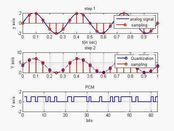
subplot(3,1,1);
plot(t,x,'linewidth',2);
title('step 1');
ylabel('y axis');
xlabel('t(in sec)');
hold on;
stem(ts,xs,'r','linewidth',2)
hold off;
legend('analog signal',' sampling');
subplot(3,1,2);
stem(ts,x1,'linewidth',2)
title('step 2');
ylabel('Y axis');
hold on;
stem(ts,xq,'r','linewidth',2);
plot(ts,xq,'--r');
plot(t,(x+A)*L/(2*A),'--b');
grid;
hold off;
legend('Quantization','sampling');
subplot(3,1,3);
stairs([y y(length(y))],'linewidth',2)
title('PCM');
ylabel('Y axis');
xlabel('bits');
axis([0 length(y) -2 2]);
grid on;
OUTPUT: